Use of xmipp_wavelet_bayesian_denoising
xmipp_wavelet_bayesian_denoising is an image denoising routine especially aimed at denoising images whose noise is additive but not white (as many other denoising techniques assume).
If you find this routine helpful please cite the article:
C.O.S.Sorzano, E. Ortiz, M. López, J. Rodrigo. Improved Bayesian image denoising based on wavelets with applications to Electron Microscopy. Pattern Recognition, 39: 1205-1213 (2006) http://biocomp.cnb.uam.es/~coss/Articulos/Sorzano2006.pdf
For running this routine you will need the free library WaveLab 850. You may get it from http://www-stat.stanford.edu/~wavelab
This routine is the MATLAB version of the C++ one implemented in the Image package Xmipp C.O.S.Sorzano, R. Marabini, J. Velázquez-Muriel, J.R. Bilbao-Castro, S.H.W. Scheres, J.M. Carazo, A. Pascual-Montano. XMIPP: a new generation of an open-source image processing package for Electron Microscopy. Journal of Structural Biology 148: 194-204 (2004) http://biocomp.cnb.uam.es/~coss/Articulos/Sorzano2004d.pdf
In this document we will show how to use this routine and some results obtained with it.
Follow these links to get the data and program:
Data: http://biocomp.cnb.uam.es/~coss/Programs/xmipp_wavelet_bayesian_denoising/Bacteriorhodpsin_projection.tif http://biocomp.cnb.uam.es/~coss/Programs/xmipp_wavelet_bayesian_denoising/experimental_micrograph.tif
Contents
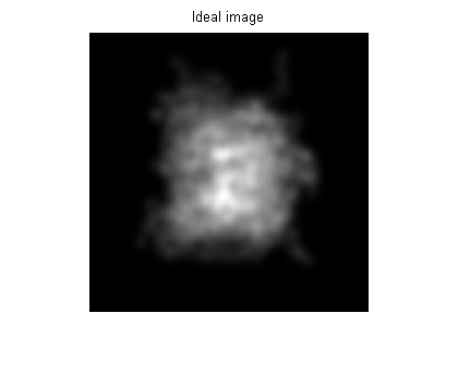
Loading an image
Iideal=im2double(imread('Bacteriorhodpsin_projection.tif'));
imshow(Iideal, [min(Iideal(:)) max(Iideal(:))]); title('Ideal image');
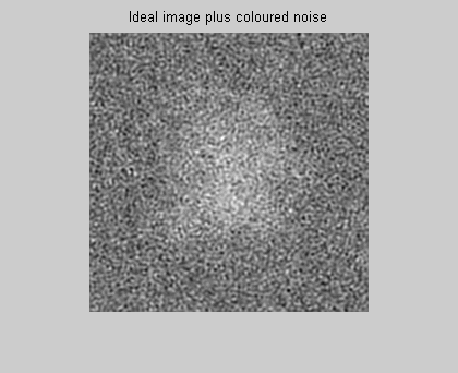
Add white noise and non-white noise
white_noise=randn(size(Iideal));

% Low pass filter noise
noise_max_freq=0.5; % White noise has a maximum frequency of 1
b = remez(10,[0 noise_max_freq-0.1 noise_max_freq+0.1 1],[1 1 0 0]);
h = ftrans2(b);
coloured_noise=imfilter(white_noise,h);
Ncoloured=var(coloured_noise(:));
coloured_noise=coloured_noise/sqrt(Ncoloured);

% Add the noise with a given SNR
SNR=1/3;
S=var(Iideal(:));
Iwhite=Iideal+sqrt(S/SNR)*white_noise;
Icoloured=Iideal+sqrt(S/SNR)*coloured_noise;
figure
imshow(Iwhite, [min(Iwhite(:)) max(Iwhite(:))]); title('Ideal image plus white noise');
figure
imshow(Icoloured, [min(Icoloured(:)) max(Icoloured(:))]); title('Ideal image plus coloured noise');

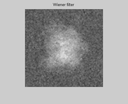
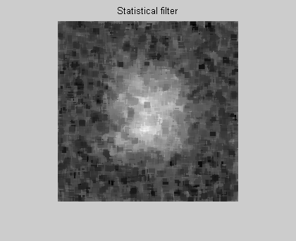
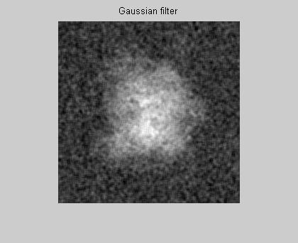
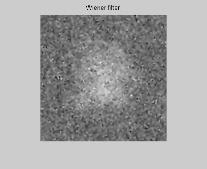
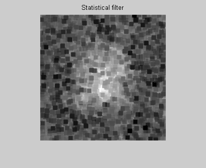
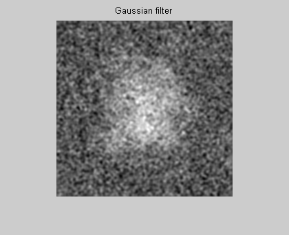
Denoise the white noise image with other approaches
Ifiltered=wiener2(Iwhite,[5 5]);
figure
imshow(Ifiltered, [min(Ifiltered(:)) max(Ifiltered(:))]); title('Wiener filter');
Ifiltered=medfilt2(Iwhite,[5 5]);
figure
imshow(Ifiltered, [min(Ifiltered(:)) max(Ifiltered(:))]); title('Median filter');
Ifiltered=ordfilt2(Iwhite,3,ones(9));
figure
imshow(Ifiltered, [min(Ifiltered(:)) max(Ifiltered(:))]); title('Statistical filter');
Ifiltered=imfilter(Iwhite,fspecial('gaussian',[5 5],3));
figure
imshow(Ifiltered, [min(Ifiltered(:)) max(Ifiltered(:))]); title('Gaussian filter');

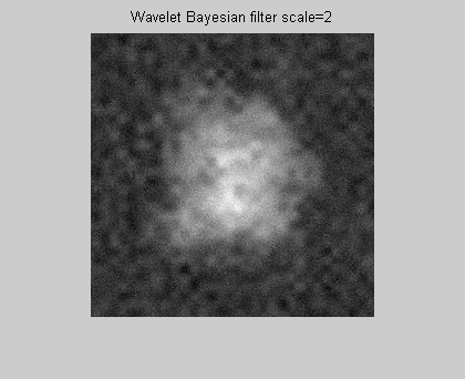
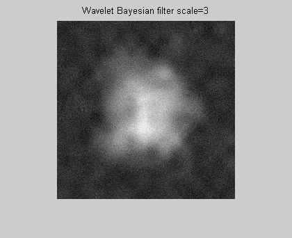
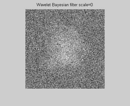
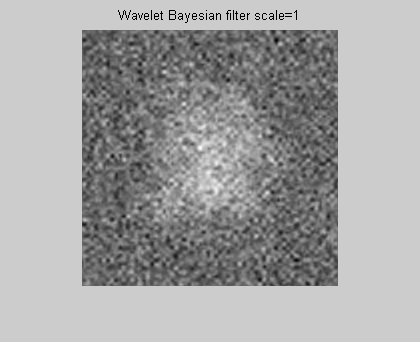
Denoise the white noise image with the wavelet bayesian denoise
To use this denoising, images must be of a size that is a power of 2. This routine has the following prototype:
Ifiltered=xmipp_wavelet_bayesian_denoising(Inoisy, allowed_scale, SNR0, SNRF)
SNR0 and SNRF are bounds for the SNR on the whole image, that is, SNR0<=SNR<=SNRF
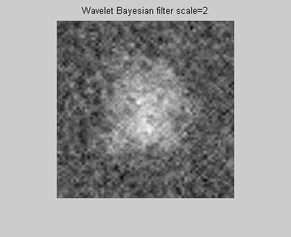
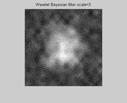
allowed_scale is a parameter that tells the routine how deep it should go in the denoising. Scale=0 indicates that only the finer details must be filtered. Scale=1 indicates that the finest two wavelet scales must be filtered, scale=2 the finest three scales, etc.
As it can be seen the more scales you filter, the more lowpass is the output
Ifiltered=xmipp_wavelet_bayesian_denoising(Iwhite,0,0.3,0.35);
figure
imshow(Ifiltered, [min(Ifiltered(:)) max(Ifiltered(:))]); title('Wavelet Bayesian filter scale=0');
Ifiltered=xmipp_wavelet_bayesian_denoising(Iwhite,1,0.3,0.35);
figure
imshow(Ifiltered, [min(Ifiltered(:)) max(Ifiltered(:))]); title('Wavelet Bayesian filter scale=1');
Ifiltered=xmipp_wavelet_bayesian_denoising(Iwhite,2,0.3,0.35);
figure
imshow(Ifiltered, [min(Ifiltered(:)) max(Ifiltered(:))]); title('Wavelet Bayesian filter scale=2');
Ifiltered=xmipp_wavelet_bayesian_denoising(Iwhite,3,0.3,0.35);
figure
imshow(Ifiltered, [min(Ifiltered(:)) max(Ifiltered(:))]); title('Wavelet Bayesian filter scale=3');


Repeating the experiment with coloured noise
Ifiltered=wiener2(Icoloured,[5 5]);
figure
imshow(Ifiltered, [min(Ifiltered(:)) max(Ifiltered(:))]); title('Wiener filter');
Ifiltered=medfilt2(Icoloured,[5 5]);
figure
imshow(Ifiltered, [min(Ifiltered(:)) max(Ifiltered(:))]); title('Median filter');
Ifiltered=ordfilt2(Icoloured,3,ones(9));
figure
imshow(Ifiltered, [min(Ifiltered(:)) max(Ifiltered(:))]); title('Statistical filter');
Ifiltered=imfilter(Icoloured,fspecial('gaussian',[5 5],3));
figure
imshow(Ifiltered, [min(Ifiltered(:)) max(Ifiltered(:))]); title('Gaussian filter');
Ifiltered=xmipp_wavelet_bayesian_denoising(Icoloured,0,0.3,0.35);
figure
imshow(Ifiltered, [min(Ifiltered(:)) max(Ifiltered(:))]); title('Wavelet Bayesian filter scale=0');
Ifiltered=xmipp_wavelet_bayesian_denoising(Icoloured,1,0.3,0.35);
figure
imshow(Ifiltered, [min(Ifiltered(:)) max(Ifiltered(:))]); title('Wavelet Bayesian filter scale=1');
Ifiltered=xmipp_wavelet_bayesian_denoising(Icoloured,2,0.3,0.35);
figure
imshow(Ifiltered, [min(Ifiltered(:)) max(Ifiltered(:))]); title('Wavelet Bayesian filter scale=2');
Ifiltered=xmipp_wavelet_bayesian_denoising(Icoloured,3,0.3,0.35);
figure
imshow(Ifiltered, [min(Ifiltered(:)) max(Ifiltered(:))]); title('Wavelet Bayesian filter scale=3');

Applications in Electron Microscopy
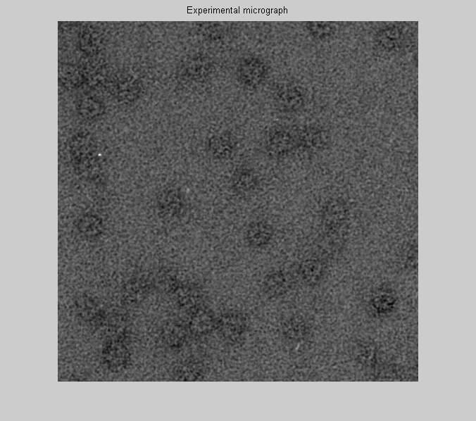
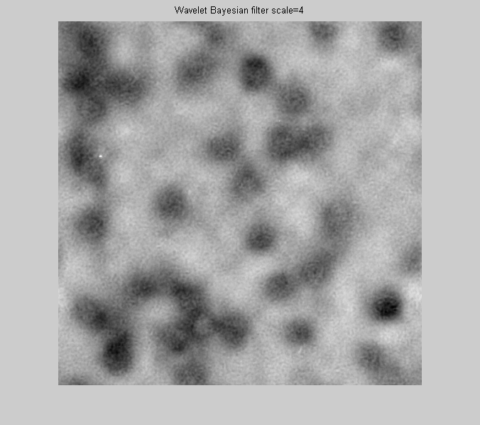
This algorithm is especially suited for particle picking and prealignment in Electron Microscopy of macromolecular complexes Here you are an example of micrograph denoising using experimental data
Inoisy=im2double(imread('Experimental_micrograph.tif'));
imshow(Inoisy, [min(Inoisy(:)) max(Inoisy(:))]); title('Experimental micrograph');
Ifiltered=xmipp_wavelet_bayesian_denoising(Inoisy,4,0.2,0.25);
figure
imshow(Ifiltered, [min(Ifiltered(:)) max(Ifiltered(:))]); title('Wavelet Bayesian filter scale=4');
Finish the program
close all